This note is a record of my presentation script of my talk on convex bodies approximation for the seminar: convex geometry.
1. John’s Ellipsoid
Outline:
In this part, I want to start by introducing John’s ellipsoid theorem, one of the most famous results in this field, by showing some examples in both asymmetric and symmetric cases in 2D.
Then I will discuss Theorem 1.2 and Theorem 1.3 in more detail, and give the proofs on the blackboard. I will skip the proof of Lemma 1.1 as well as the explanation of tensor product used in the proof.
Later, I will introduce the important concept of John’s position and show a simple illustration.
Finally, I will briefly mention the definition of Banach–Mazur distance and state Theorem 1.4 with its proof—just to give a sense of the idea behind John’s ellipsoid theorem mentioned at the beginning.
Lemma 1.1
Let
$$ \mathcal{D} = { A \in \mathcal{P} : \det(A) \geq 1 } $$
Then \( \mathcal{D} \) is a closed, smooth, and strictly convex subset of \( \mathcal{P} \), with non-empty interior.
Proof of Lemma 1.1
Let \( A = I \in \mathcal{D} \Rightarrow \mathcal{D} \neq \emptyset \), hence \( \mathcal{D} \) has non-empty interior.
It is clear that \( \mathcal{D} \) is closed and smooth.
To prove convexity, it suffices to show that the function \( f(A) = \log \det A \) is concave. Then:
$$ \log \det (\lambda A + (1 - \lambda) B) \geq \lambda \log \det A + (1 - \lambda) \log \det B $$
which implies:
$$ \det(\lambda A + (1 - \lambda) B) \geq (\det A)^\lambda (\det B)^{1 - \lambda} $$
Thus, if \( A, B \in \mathcal{D} \), then \( \det(\lambda A + (1 - \lambda) B) \geq 1 \), so \( \lambda A + (1 - \lambda) B \in \mathcal{D} \), and convexity holds.
To show that \( f(A) = \log \det A \) is concave, we compute its second derivative.
- Define:
\[ f(t) := \log \det(A + tH), \quad t \in (-\varepsilon, \varepsilon), \quad A \in \mathcal{P}, \quad H \in \mathrm{Sym}_n \]
- Compute the first derivative:
$$ f’(t) = \frac{d}{dt} \log \det(A + tH) = \mathrm{tr}\left( (A + tH)^{-1} H \right) $$
- Compute the second derivative:
$$ f’’(t) = \frac{d}{dt} , \mathrm{tr}\left( (A + tH)^{-1} H \right) = \mathrm{tr}\left( - (A + tH)^{-1} H (A + tH)^{-1} H \right) $$
$$ = -\mathrm{tr}\left( \left[ (A + tH)^{-1} H \right]^2 \right) < 0 $$
with equality if and only if \( H = 0 \).
Therefore, \( f \) is strictly concave, and so \( \mathcal{D} \) is strictly convex.
Theorem: Uniqueness of Maximum Volume Inner Ellipsoid
If \( C \subset \mathbb{R}^d \) is a convex body, then the inner ellipsoid of maximal volume is unique.
Proof of Theorem 1.2
There exists at least one ellipsoid in \( C \) of maximum volume since \( C \) is compact.
We prove this by contradiction. Suppose there are two distinct maximum volume ellipsoids inside \( C \).
Without loss of generality, assume their volumes are equal to that of the unit ball \( B^d \). These ellipsoids can be written as \( AB^d \) and \( BB^d \), for suitable matrices \( A, B \in \mathcal{P} \), where \( A \neq B \) and \( \det A = \det B = 1 \).
By the convexity of \( C \), we have:
$$ \frac{1}{2}(A + B)B^d \subseteq C $$
But from Lemma 1.1, we know that:
$$ \det\left( \frac{1}{2}(A + B) \right) > \frac{1}{2} \det A + \frac{1}{2} \det B = 1 $$
This means the ellipsoid:
$$ \frac{1}{2}(A + B)B^d $$
has greater volume than both \( AB^d \) and \( BB^d \), contradicting the assumption that they are of maximum volume.
Therefore, the maximum volume ellipsoid inside \( C \) is unique. □
Theorem (John’s Characterization)
Let \( C \in \mathcal{C}_p \) be a convex body that is origin-symmetric (i.e., \( x \in C \Rightarrow -x \in C \)), and suppose that \( B^d \subseteq C \). Then the following are equivalent:
- \( B^d \) is the unique John’s ellipsoid in \( C \).
- There exist vectors \( u_i \in B^d \cap \partial C \) and weights \( \lambda_i > 0 \), for \( i = 1, \dots, m \), with \( d \leq m \leq \frac{1}{2}d(d + 1) \), such that:
$$ I = \sum \lambda_i , u_i \otimes u_i \quad \text{and} \quad \sum \lambda_i = d $$
Here, \( \otimes \) denotes the outer product of vectors.
Proof sketch of this theorem
Proof of Theorem 1.3
(i) ⇒ (ii):
The set of all ellipsoids inside \( C \) can be represented as:
$$ \mathcal{E} = { A \in \mathcal{P} : A u \cdot v \leq h_C(v) \text{ for all } u, v \in \partial B^d } $$
A key step is to rewrite \( A u \cdot v \) as \( A \cdot (u \otimes v) \), since:
$$ \langle A u, v \rangle = (A u)^T v = \sum_{i=1}^d \left( \sum_{j=1}^d A_{ij} u_j \right) v_i = \sum_{i,j} A_{ij} u_j v_i $$
and
$$ \langle A, u \otimes v \rangle = \sum_{i,j} A_{ij} u_i v_j $$
Because \( A \) is symmetric, these expressions are equal. This reformulation expresses the “quadratic form” as linear constraints in matrix space. Thus, \( \mathcal{E} \) is the intersection of the family of closed halfspaces:
$$ { A \in \mathbb{E}^{\frac{1}{2}d(d+1)} : A \cdot (u \otimes v) \leq h_C(v) } \quad \text{for } u, v \in \partial B^d \tag{1} $$
From assumption (i), we know:
- \( \det A < 1 \) for all \( A \in \mathcal{E} \setminus {I} \)
- \( \mathcal{E} \) is convex
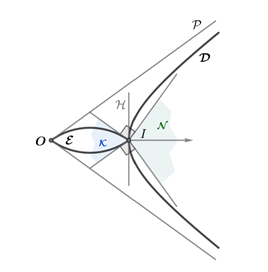
- \( \mathcal{D} \cap \mathcal{E} = {I} \), and \( \mathcal{E} \) is separated from \( \mathcal{D} \) by the unique support hyperplane \( \mathcal{H} \) of \( \mathcal{D} \) at \( I \)
Now consider the support cone \( \mathcal{K} \) of \( \mathcal{E} \) at \( I \), which helps us construct the normal cone \( \mathcal{N} \). From (1), \( \mathcal{E} \) is an intersection of halfspaces in \( \mathcal{P} \), so \( \mathcal{K} \) is the intersection of those halfspaces whose boundaries contain \( I \), i.e.,
$$ I \cdot (u \otimes v) = u \cdot v = h_C(v) $$
But since:
\[ u \cdot v \leq 1, \quad B^d \subset C \Rightarrow 1 = h_{B^d}(v) \leq h_C(v) \]
the equality \( u \cdot v = h_C(v) \) only holds when \( u = v \).
Thus, \( \mathcal{K} \) is the intersection of the following halfspaces:
$$ { A \in \mathbb{E}^{\frac{1}{2}d(d+1)} : A \cdot (u \otimes u) \leq 1 } \quad \text{for } u \in B^d \cap \partial C \tag{2} $$
The normal cone \( \mathcal{N} \) of \( \mathcal{E} \) at \( I \) is the polar cone of \( \mathcal{K} - I \), which gives:
$$ \mathcal{N} = \text{pos} { u \otimes u : u \in B^d \cap \partial C } $$
So \( I \in \mathcal{N} \).
By Carathéodory’s theorem, there exist \( u_i \in B^d \cap \partial C \), \( \lambda_i > 0 \), with \( i = 1, \dots, m \), and \( m \leq \frac{1}{2}d(d+1) \), such that:
$$ I = \sum_i \lambda_i u_i \otimes u_i $$
and
$$ d = \text{tr}(I) = \sum_i \lambda_i , \text{tr}(u_i \otimes u_i) = \sum_i \lambda_i $$
Also, \( m \geq d \) is clear, since at least \( d \) linearly independent vectors are needed to span \( \mathbb{E}^d \).
(ii) ⇒ (i):
Using the same definitions of \( \mathcal{N}, \mathcal{K}, \mathcal{E} \), assumption (ii) implies \( I \in \mathcal{N} \),
so the hyperplane \( \mathcal{H} \) through \( I \), orthogonal to \( I \), separates \( \mathcal{K} \) from \( \mathcal{D} \).
By convexity, this implies:
$$ \mathcal{D} \cap \mathcal{E} = { I } $$
which shows that \( \det A < 1 \) for all \( A \in \mathcal{E} \setminus {I} \), which is exactly statement (i).
Corollary 1.4
Let \( | \cdot | \) be the Euclidean norm and \( | \cdot | \in \mathcal{N}(\mathbb{E}^d) \) be any norm. Then the Banach–Mazur distance satisfies:
$$ \delta^{BM}(| \cdot |, | \cdot |) \leq \sqrt{d} $$
Proof
Assume \( T \) is chosen such that \( B^d \subseteq T B_{| \cdot |} \), and \( T B_{| \cdot |} \) is the maximum volume ellipsoid inside \( C = T B_{| \cdot |} \).
This gives the left-hand inclusion in the definition of Banach–Mazur distance.
Now we need to show the right-hand inclusion:
$$ C = T B_{| \cdot |} \subseteq \sqrt{d} , B^d $$
Choose \( u_i, \lambda_i \) as in Theorem 1.3, so that:
$$ I = \sum_i \lambda_i , u_i \otimes u_i, \quad \sum_i \lambda_i = d \tag{5} $$
Since \( u_i \in B^d \cap \partial C \), it follows that:
- \( C \) lies in the support halfspace of \( B^d \) at each \( u_i \),
- So for all \( x \in C \), we have \( u_i \cdot x \leq 1 \)
Now represent \( x \) using (5):
$$ x = I x = \sum_i \lambda_i (u_i \otimes u_i) x = \sum_i \lambda_i (u_i \cdot x) u_i $$
Then compute its Euclidean norm:
$$ |x|^2 = x \cdot x = \sum_i \lambda_i (u_i \cdot x)^2 \leq \sum_i \lambda_i = d \quad \text{for all } x \in T B_{| \cdot |} $$
Therefore:
$$ T B_{| \cdot |} \subseteq \sqrt{d} , B^d $$
This proves the upper bound \( \delta^{BM}(| \cdot |, | \cdot |) \leq \sqrt{d} \).
2. Reverse Isoperimetric Inequality
Outline:
In this section, I would like to talk about an important application of John’s Characterization Theorem: the reverse isoperimetric inequality.
I will start by introducing the classical isoperimetric inequality and the definition of the isoperimetric quotient. Then, I will present Theorem 2.1 and show how the volume, surface area, and isoperimetric quotient behave for the ball and cube as the dimension \( d \) increases. Finally, I will sketch a proof of Theorem 2.1.
Theorem 2.1
Let \( C \in \mathcal{C}_p \) be a convex body symmetric about the origin, and let \( T \) be a linear transformation that places \( C \) in John’s position. Then:
$$ \frac{S(TC)}{V(TC)^{\frac{d-1}{d}}} \leq 2d $$
with equality if and only if \( C \) is a parallelotope.
Proof
Choose a linear transformation \( T \) such that \( B^d \) is the maximum volume ellipsoid inside \( TC \). We will show:
$$ V(TC) \leq 2^d \tag{6} $$
Let \( u_i, \lambda_i \) be the vectors and coefficients from Theorem 1.3, and define the convex body:
$$ D = \left{ x \in \mathbb{R}^d : |u_i \cdot x| \leq 1,\quad i = 1, \dots, m \right} $$
For each \( i \), define the function:
$$ f_i(t) := \chi_{[-1,1]}(t) = \begin{cases} 1, & \text{if } |t| \leq 1 \ 0, & \text{otherwise} \end{cases} $$
Then the function
$$ x \mapsto \prod_i f_i(u_i \cdot x)^{\lambda_i} $$
is the characteristic function of \( D \). We integrate this over \( \mathbb{R}^d \):
$$ V(D) = \int_{\mathbb{R}^d} \chi_D(x) , dx = \int_{\mathbb{R}^d} \prod_i f_i(u_i \cdot x)^{\lambda_i} dx $$
By the Brascamp–Lieb inequality, we get:
$$ \int_{\mathbb{R}^d} \prod_i f_i(u_i \cdot x)^{\lambda_i} dx \leq \prod_i \left( \int_{\mathbb{R}} f_i(t) dt \right)^{\lambda_i} $$
Since \( f_i \) is the indicator function of \( [-1,1] \), each integral is:
$$ \int_{\mathbb{R}} f_i(t) dt = 2 $$
So:
$$ V(D) \leq \prod_i 2^{\lambda_i} = 2^{\sum_i \lambda_i} = 2^d $$
Since \( TC \subseteq D \), this proves inequality (6).
Now using the definition of Minkowski surface area and the inclusion \( B^d \subseteq TC \), we get:
$$ S(TC) = \lim_{\varepsilon \to 0^+} \frac{V(TC + \varepsilon B^d) - V(TC)}{\varepsilon} \leq \lim_{\varepsilon \to 0^+} \frac{V(TC + \varepsilon TC) - V(TC)}{\varepsilon} = d \cdot V(TC) $$
Using (6):
$$ S(TC) \leq d \cdot V(TC) \leq 2d \cdot V(TC)^{\frac{d-1}{d}} $$
which completes the proof. □
3. Asymptotic Best Approximation by Polytopes
Outline:
In this section, I’ll talk about how the difference between a convex body and its approximation by an \( n \)-facet polytope behaves as the dimension \( d \) grows large.
We start with the classic example: approximating a Euclidean ball (or ellipsoid) using polytopes with a fixed number of facets. In dimension \( d = 2 \), this is relatively simple (e.g., using regular polygons), but in dimensions \( d > 2 \), the problem becomes significantly harder. I’ll briefly mention some known results from the literature without going into full technical detail.
Then I’ll present an asymptotic formula that gives insight into the best achievable approximation error in high dimensions. While the proof is complex, I’ll only explain the strategy and core ideas to provide some intuition.
After that, I will highlight how the classic isoperimetric inequality for convex polytopes can be viewed as a consequence or application of this result.
Finally, I’ll mention an inscribed version of the main theorem, which will be useful in the next (and final) section.
4. Heuristic Principle
Outline:
In this final section, I’ll introduce the famous heuristic principle in convex geometry.
This principle is based on the observation that random polytope approximations (e.g., taking the convex hull of random points on the boundary of a convex body) can perform surprisingly well—even comparable to the best possible deterministic approximations—as the dimension increases.
I’ll present a known result from the literature that quantifies this error, showing that in high dimensions, the difference between the optimal polytope approximation and the random one becomes negligible in many cases.
This illustrates a broader geometric insight: in high-dimensional settings, random constructions can be nearly as good as optimal, offering simpler and more flexible approaches to approximation problems.