This post is a record for my project “classic-optimization-methods-lab”, where I implemented and compared three classic optimization algorithms: Gradient Descent with line search, Newton’s method, and BFGS. These methods form the foundation of numerical optimization, and I wanted to see how they behave on several test problems in practice — not just in theory.
1 Introduction
In this project, I implemented three classic optimization methods: Gradient Descent, Newton’s Method, and BFGS. All three use a common backtracking line search routine to determine the step size at each iteration. First I want to recall a little bit of the three methods. Below is a brief overview of each algorithm and how it was implemented.
1.1 Gradient Descent with Line Search
Gradient descent updates the current point using the negative gradient direction:
\[ x_{k+1} = x_k - \alpha_k \nabla f(x_k) \]
Here, \( \alpha_k \) is the step size determined using backtracking line search to satisfy the Armijo condition:
\[ f(x + \alpha p) \leq f(x) + c \alpha \nabla f(x)^\top p \]
where \( p = -\nabla f(x) \) is the steepest descent direction. The Python code I used is:
c = 0.1
tau = 0.8
alpha_init = 1.0

alpha = alpha_init
while f(x + alpha * p) > f(x) + c * alpha * np.dot(grad_f(x), p):
    alpha *= tau
return alpha
This method is easy to implement and works reliably, but it may converge slowly—especially on ill-conditioned functions like Rosenbrock.
1.2 Newton’s Method
Newton’s method uses second-order derivatives to speed up convergence by approximating the function locally as a quadratic. At each iteration, it directly jumps towards the local minimum of this approximation:
\[ x_{k+1} = x_k - \alpha_k \left[ \nabla^2 f(x_k) \right]^{-1}\nabla f(x_k) \]
Here, \( \nabla^2 f(x_k) \) is the Hessian matrix (second-order derivatives). In practice, instead of explicitly computing the inverse Hessian, we solve the linear system:
\[ \nabla^2 f(x_k) p_k = -\nabla f(x_k) \]
In my implementation, I used a straightforward Newton step without line search (setting \(\alpha_k = 1\)), meaning the update directly follows the solved direction. While simple and extremely fast when close to the solution, this approach can struggle if the starting point is far or the Hessian is ill-conditioned.
1.3 BFGS Method
The BFGS method is a popular quasi-Newton approach that approximates the Hessian matrix iteratively, avoiding direct computation of second derivatives. At each iteration, it updates the approximate inverse Hessian \( H_k \) using gradient differences.
The update step is given by:
\[ x_{k+1} = x_k + \alpha_k p_k,\quad \text{where } p_k = -H_k \nabla f(x_k) \]
I used a backtracking line search with Armijo condition (same as gradient descent), initializing \(\alpha = 1.0\), and reducing it by \(0.8\) each iteration if needed.
If the curvature condition \(\mathbf{y}_k^\top \mathbf{s}_k > 10^{-10}\) fails, the algorithm terminates early to avoid numerical instability.
2 Test Problems & Setup
I tested the optimization methods on two classic problems:
Rosenbrock function (nonconvex, challenging for gradient-based methods): \[ f(x, y) = (1 - x)^2 + 100(y - x^2)^2 \]
Quadratic function (convex, ideal for testing Newton’s method): \[ f(x, y) = x^2 + 2y^2 \]
Setup:
- Initial point: \((0, 0)\)
- Tolerance: \(|\nabla f(x)| \leq 10^{-6}\)
- Maximum iterations: 100
- Metrics recorded: Objective values, gradient norms, and iteration count.
3 Results & Observations
Rosenbrock Function
Starting from the initial point \((0,0)\):
| Method | Iterations | Converged? | Final Point | Objective |
|---|---|---|---|---|
| Gradient Descent | 1000 | No (slow) | \((0.903, 0.815)\) | 0.0095 |
| Newton | 2 | Yes (fast) | \((1.000, 1.000)\) | 0.0000 |
| BFGS | 22 | Yes | \((1.000, 1.000)\) | 0.0000 |
Observations:
- Newton’s method rapidly converged in only 2 iterations, finding the exact minimum.
- BFGS also converged quickly (22 iterations), though it triggered a curvature condition warning, indicating numerical sensitivity.
- Gradient Descent was very slow, unable to fully converge even after 1000 iterations.
Quadratic Function
Starting from the initial point \((3,4)\):
| Method | Iterations | Converged? | Final Point | Objective |
|---|---|---|---|---|
| Gradient Descent | 37 | Yes | \((9.85\ast 10^{-28}, -2.46\ast 10^{-07})\) | ≈0 |
| Newton | 1 | Yes (fast) | \((0.000, 0.000)\) | 0.0000 |
| BFGS | 7 | Yes | \((-9.91\ast 10^{-07}, -4.40\ast 10-07)\) | ≈0 |
Observations:
- Newton’s method again converged immediately after 1 iteration.
- BFGS quickly reached a very accurate solution in just 7 iterations, despite a curvature warning.
- Gradient Descent converged reliably, though slower, taking 37 iterations.
Key Takeaways:
- Newton’s method provides the fastest convergence near optima, but requires the Hessian and has higher computational cost.
- BFGS balances computational efficiency and convergence speed effectively, making it a common choice in practice.
- Gradient Descent is simple but significantly slower, particularly on challenging functions like Rosenbrock.
The plots further illustrate these differences clearly. You can click on the link and check them in my projects.
4 Conclusion
In this short project, I explored three foundational optimization algorithms—Gradient Descent, Newton’s Method, and BFGS. While Newton’s method excels near optima with rapid convergence, BFGS offers a robust and efficient alternative without explicit second derivatives. Gradient Descent, though simpler, often requires significantly more iterations. This experience underscored the practical trade-offs of choosing optimization methods, highlighting BFGS as a versatile and reliable option for typical use cases. For codes and detailed experiments and results please be free to check on my project. Again it’s not a formal project and I am plan to add more methods that the textbook didn’t mentioned but useful in practice to it and also extend this post. If you have any questions or any thoughts, please contact me via e-mails or start a issue in that repository. Thank you for reading!
(Update Part) Demonstration: KKT Conditions and the Penalty Method
To demonstrate an understanding of constrained nonlinear optimization, this project includes a demo solving a problem and verifying it against the Karush-Kuhn-Tucker (KKT) conditions.
The Problem
- Minimize: \(f(x, y) = (x - 2)² + (y - 2)²\)
- Subject to: \(g(x, y) = x² + y² - 1 ≤ 0\)
The analytical solution, found by applying the KKT conditions, is \((x, y) = (1/√2, 1/√2)\).
The Numerical Method
The problem was solved numerically using the Penalty Method. This transforms the constrained problem into a series of unconstrained problems of the form: \[ P(x) = f(x) + ρ * max(0, g(x))² \]
This new problem \(P(x)\) was then solved using the implemented Gradient Descent algorithm for increasing values of the penalty parameter \(ρ\).
Results
Original test and the problems
As \(ρ\) increases, the numerical results are shown in the following table: (see in log03)
| Rho (ρ) | Numerical Solution | Error (Distance to KKT point) | Converged Iterations |
|---|---|---|---|
| 1 | [0.89816091, 0.89816095] | 0.270191 | 31 iterations |
| 10 | [0.73679149, 0.73679161] | 0.041981 | 123 iterations |
| 100 | [0.71030916, 0.71030929] | 0.004529 | 1087 iterations |
| 1000 | [0.70099022, 0.71383061] | 0.009090 | not coverged in max_iter |
| 10000 | [0.5330758, 0.84608049] | 0.222712 | not coverged in max_iter |
As we can notice, the numerical solution didn’t converges to the true KKT point as \(ρ\) increases after 100. Conversely it behaves even worse when \(ρ\) rises to 10000.
We can see the issue clearly by this following plot:
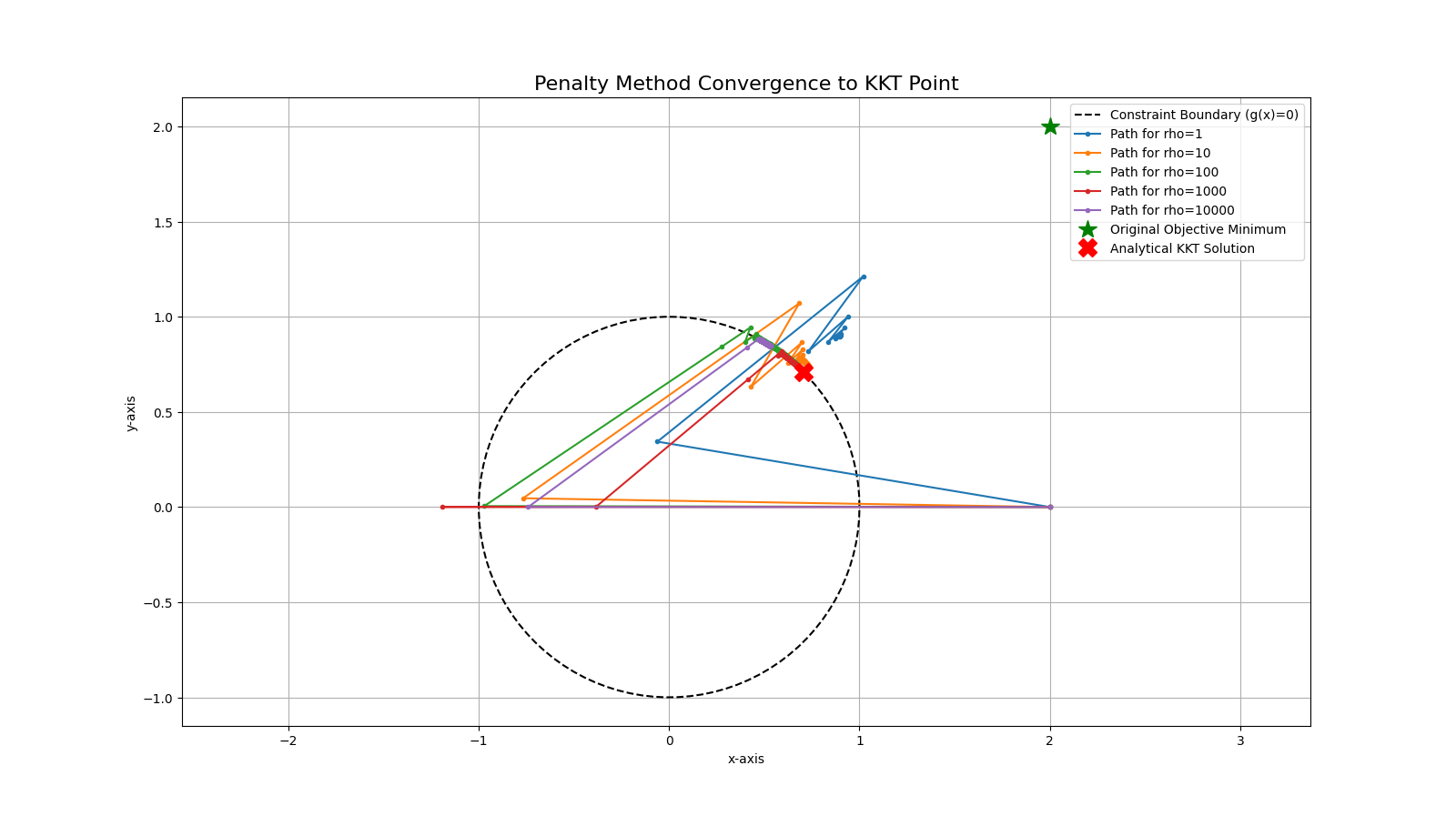
This was because the Hessian matrix of this penalized objective function P(x) becomes increasingly ill-conditioned when we increase the penalty parameter \(ρ\).
- When we have a low \(ρ\), the objective function looks like a smooth valley (f(x)), with a gentle, sloping penalty wall that starts at the constraint boundary, and the optimizer can easily find its way down the slope and settle at the bottom;
- But when \(ρ\) goes very high, The original valley \(f(x)\) is now almost irrelevant. The landscape is dominated by the penalty term \(ρ * max(0, g(x))²\). This creates an incredibly steep wall—almost a vertical cliff—at the constraint boundary \(g(x) = 0\).
More specifically:
- Just one step outside the feasible region (the unit circle), the gradient of the penalty term becomes enormous \(2 * ρ * g(x) * grad_g(x)\).
- The algorithm calculates the huge gradient, which points sharply inwards. The search direction \(p\) = -gradient is a massive vector pointing across the valley.
- The update step \(x + alpha * p\) causes the algorithm to leap completely over the narrow feasible region and land on the other side of the canyon wall. In the next iteration, it sees another huge gradient pointing back in the opposite direction. The optimizer starts bouncing from one side of the constraint boundary to the other, never settling in the middle.
- Tiny Step Sizes: The backtracking line search tries to prevent this. It sees that a full step (alpha = 1.0) makes the objective value much worse (because it overshot). So, it starts shrinking alpha (alpha *= 0.8). To make any progress in such a steep canyon, it has to shrink alpha to a minuscule value.
- The algorithm is still making progress, but each step is now incredibly tiny. It is crawling down the canyon wall so slowly that it exhausts the max_iter limit before it can reach the tolerance tol.
That leads to the technique which I used to fix it.
Enhancement test
Use a warm start. The solution for \(\rho=100\) is a very good starting point for the \(\rho=1000\) problem. This is a standard technique in numerical optimization. Just look like this:
x0 = np.array([2.0, 0.0]) # Initial starting point
last_solution = x0

for rho in rho_values:
    # ... create penalty_problem ...

    # Use the solution from the previous, easier problem as the starting point
    # for the current, harder problem. This is a "warm start".
    solution, history, _ = gradient_descent.solve(penalty_problem, last_solution, max_iter=2000)

    last_solution = solution # Update for the next loop
Then the results shown as following: (see in log04)
| Rho (ρ) | Numerical Solution | Error (Distance to KKT point) | Converged Iterations |
|---|---|---|---|
| 1 | [0.89816091, 0.89816095] | 0.270191 | 31 iterations |
| 10 | [0.73679155, 0.73679155] | 0.041981 | 41 iterations |
| 100 | [0.71030922, 0.71030922] | 0.004529 | 31 iterations |
| 1000 | [0.7074297, 0.7074297] | 0.000457 | 41 iterations |
| 10000 | [0.7071391, 0.7071391] | 0.000046 | not coverged in max_iter |
You can see the difference here. Even though when \(ρ =10000\) it still not converged, but we can see the numerical solution perfectly converges to the KKT point and Error goes to 0 as \(p\) increases.
And the plots further illustrates the difference clearly:
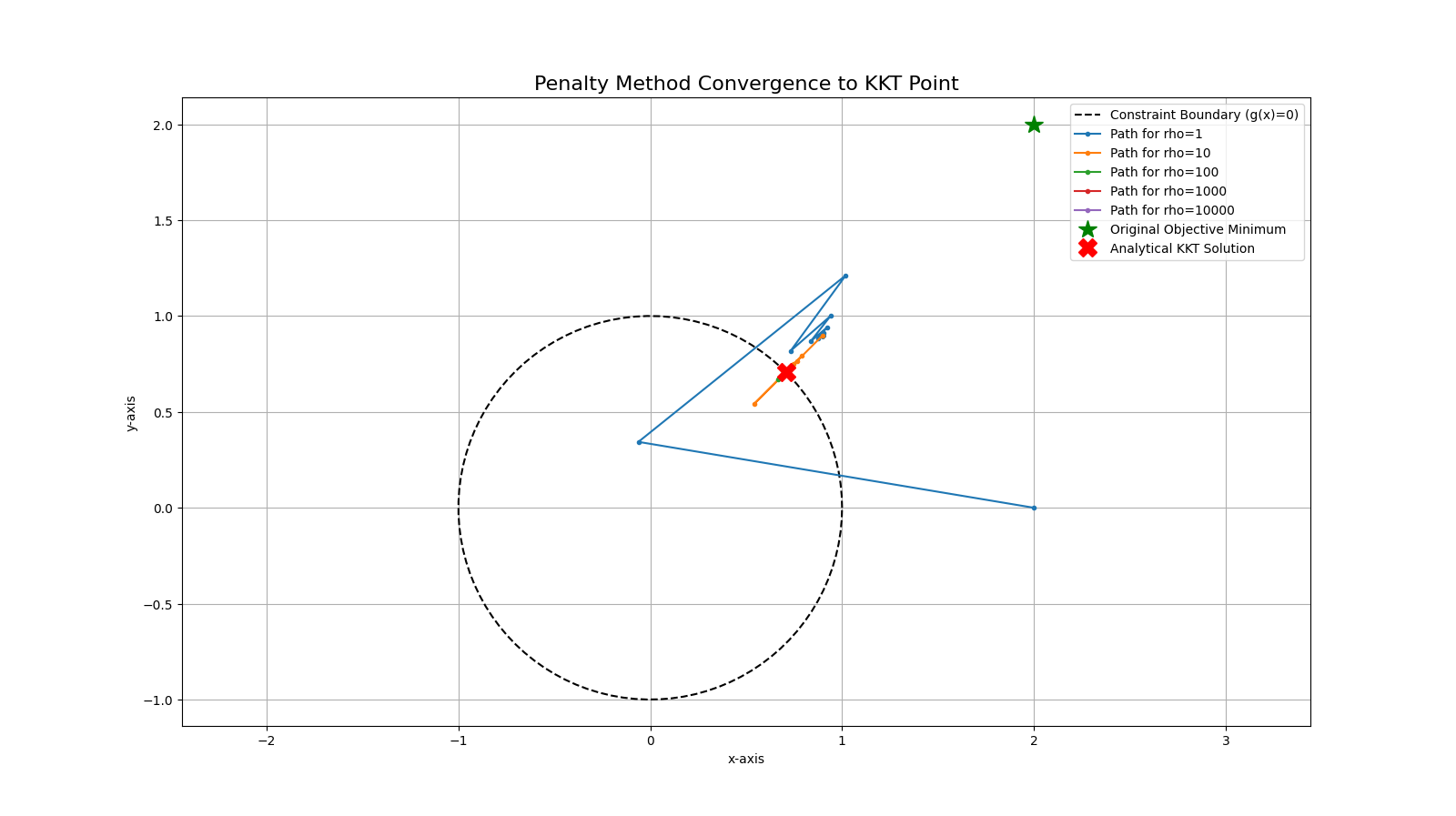
Quick summary
This demonstration shows how to solve a constrained nonlinear problem by implementing the Penalty Method. The numerical solution, found using a custom Gradient Descent solver, is shown to converge to the true optimal point derived analytically from the KKT conditions. The demonstration also highlights the practical challenge of ill-conditioning that arises with large penalty values, a key concept in numerical optimization.