As part of my effort to better understand combinatorial optimization, I’ve been going through some classic problems we covered in class. I figured it would be helpful (for myself, and maybe for others) to write down a few key ideas, along with simple Python implementations to make things more concrete. I will start the series from this post and start with the scheduling problems. Then I will talk about more about TSP problems, bin packing problems and backpack problems and so on. Mostly, this is just a way for me to organize my notes and revisit some topics.
Scheduling might sound straightforward at first—just figure out who does what, and when—but it turns out that even very basic setups can lead to surprisingly tricky problems. Many of them are NP-hard, and require clever heuristics, approximation algorithms, or even exact solvers in practice.
In this post, I’ll go over a few well-known scheduling models, starting from simple single-machine problems and gradually working up to more complex ones like job shop scheduling. I’ll keep things informal, with minimal math and maximum intuition (and a bit of code too).
1. Single-Machine Scheduling Problems
Let’s start with the simplest kind of scheduling setup: we have a single machine and a set of jobs, each with a processing time, and maybe a due date or a weight. The challenge is to decide in which order to run the jobs so that we minimize some performance metric.
Surprisingly, even this tiny setup gives rise to a variety of interesting problems. Here are a few classic ones:
1.1. Minimize the Maximum Lateness
Each job \( j \) has:
- a processing time \( p_j \)
- a due date \( d_j \)
If we schedule job \( j \) to start at time \( s_j \), its completion time is \( C_j = s_j + p_j \), and its lateness is:
\[ L_j = C_j - d_j \]
We want to minimize:
\[ L_{\max} = \max_j L_j \]
Restriction: we set each \(d_j < 0\) thus \(OPT > 0\). That’s because deciding whether there is schedule with \(L_{\max} \leq 0\) is NP-hard.
Rule: Use the Earliest Due Date (EDD) rule—schedule jobs in order of increasing \( d_j \).
This rule gives the optimal solution for minimizing \( L_{\max} \) on a single machine.
Approximation ratio: EDD is a 2-approximation algorithm which is a greedy algorithm.
1.2. Minimize Total Completion Time \( \sum C_j \)
Here we ignore due dates, and simply try to finish all jobs as early as possible. The goal is:
\[ \min \sum_{j=1}^n C_j \]
Rule: Use the Shortest Remaining Processing Time (SRPT) rule—schedule jobs from shortest to longest \( p_j \).
Approximation ratio:
If it’s preemptive schedule then SRPT is optimal. (Reason: It’s an optimal solution of the deterministic LP)
If it’s non-preemptive, then it’s a 2-approximation algorithm by LP rounding.
compute optimal preemptive schedule with SRPT
schedule each job by the order of their completion time
1.3. Minimize Weighted Completion Time \( \sum w_j C_j \)
Now each job also has a weight \( w_j \), and we care more about finishing some jobs earlier than others.
Objective:
\[ \min \sum_{j=1}^n w_j C_j \]
Rule: Consider the following LP:
$$ \begin{aligned} \min & \sum_{j=1}^n w_j C_j \\ \text{s.t.} \qquad C_j &\geq r_j + p_j \quad \forall j \in J \\ \sum_{j \in S} p_j C_j &\geq \frac{1}{2} p(S)^2 \quad \forall S \subseteq J \end{aligned} $$
Deterministic LP Rounding
If we do the following:
solve the optimal solution \(C^*\) to the LP: \( C_1^\ast \leq \dots \leq C_n^\ast \)
schedule each job according to \(C^*\): \( C_j^N := max \lbrace C_{j-1}^N, r_j \rbrace + p_j \), while \( C_1^N := r_1 + p_1 \).
Then we get:
Approximation ratio: it’s a 3-approximation algorithm.
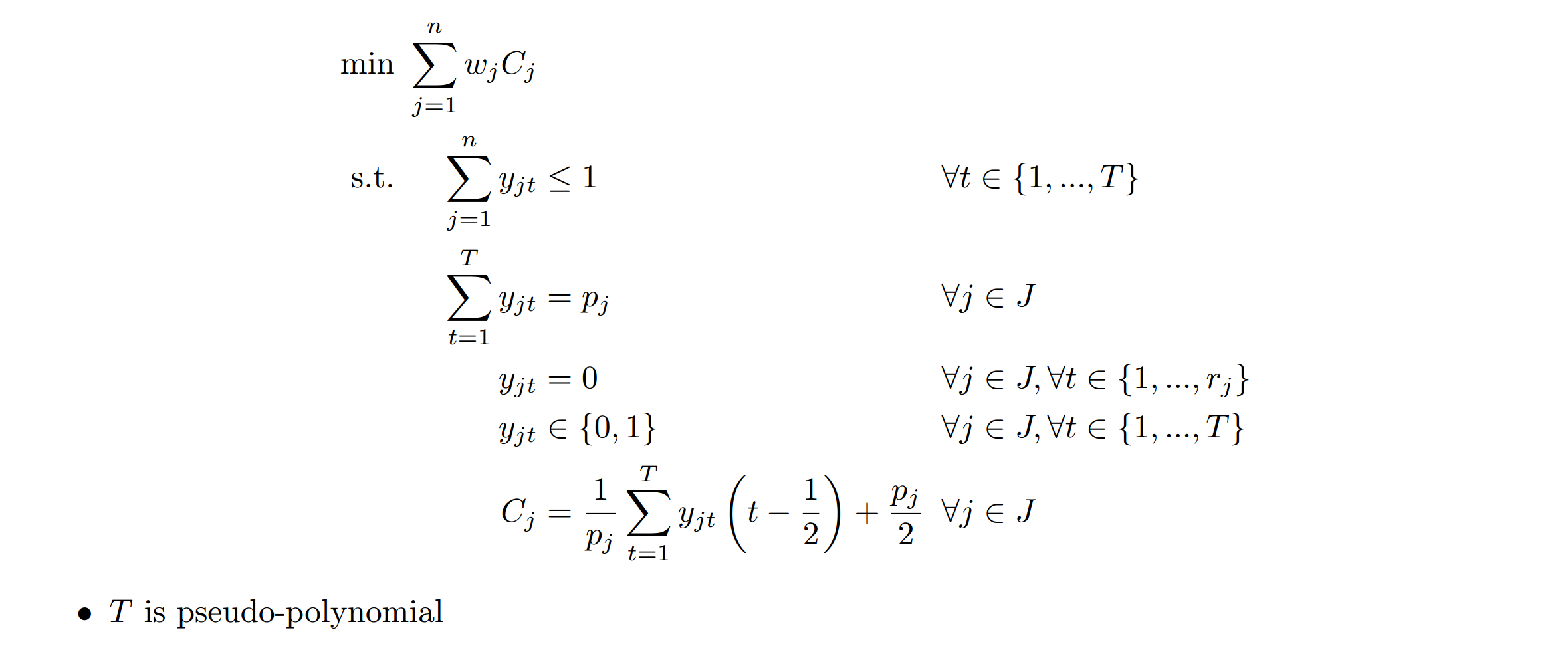
Randomized LP Rounding
Set variables \(y_{jt}\) as:
$$ y_{jt}=\begin{cases} 1 & \text{if job j is processed during time [t-1, t]}\\ 0 & \text{otherwise} \end{cases} $$
And define \(C_j\) as:
$$ C_j=\frac{1}{p_j}\sum_{t=1}^{T}y_{jt}(t-\frac{1}{2})+\frac{p_j}{2} $$
Then solve the IP relaxation:
each job j: random variable \(X_j = t - \frac{1}{2}\) with probability \(\frac{y_{jt}^\ast}{p_j}\)
reorder s.t. \(X_1 \leq \dots \leq X_n\)
schedule each job j and \(\hat{C_j} := \max\lbrace \hat{C}_{j-1}, r_j \rbrace + p_j\)
Then we get:
Approximation ratio: it’s a 2-approximation algorithm.
2. Parallel Machine Scheduling: Minimizing Makespan
After looking at single-machine scheduling, let’s turn to a more general and realistic setup: multiple machines working in parallel.
Our goal is still quite intuitive: we want to assign jobs to machines so that the last job finishes as early as possible. In other words, we want to minimize the makespan:
\[ C_{\max} = \max_{i} C_i \]
Depending on how the machines behave, the problem can be quite different. Here’s a breakdown of two classic models:
2.1. Identical Machines (Model: \( P || C_{\max} \))
In this case, we have \( m \) identical machines and \( n \) jobs. Each job \( j \) has a processing time \( p_j \), and any job can run on any machine in time \( p_j \).
Greedy Algorithm: List Scheduling
This strategy works like this:
- Sort the jobs in any order (e.g. arbitrary, or longest-first),
- Assign each job to the machine that becomes available the earliest.
Approximation ratio: The makespan produced by List Scheduling is at most:
\[ C_{\max}^{\text{LS}} \leq \left(2 - \frac{1}{m} \right) \cdot C_{\max}^{\star} \]
So it gives a (2 – 1/m)-approximation to the optimal makespan.
LPT Rule
LPT stands for Longest Processing Time first. It works like List Scheduling, but sorts jobs in decreasing \( p_j \) first.
It improves the approximation to:
\[ C_{\max}^{\text{LPT}} \leq \left( \frac{4}{3} - \frac{1}{3m} \right) \cdot C_{\max}^{\star} \]
A PTAS Using Dynamic Programming
A stronger result for this problem is: For the identical machines case (\( P ,|, C_{\max} \)), there exists a ( (1 + \varepsilon) )-approximation algorithm for any \( \varepsilon > 0 \).
The key idea is to use a dynamic programming approach, where:
- We discretize job sizes (e.g., round them to multiples of \( \varepsilon \cdot \text{OPT} \)),
- Group small jobs and large jobs,
- Use DP to pack large jobs into machines optimally (or near-optimally),
- Then assign small jobs greedily.
This gives us a PTAS (Polynomial-Time Approximation Scheme)—the runtime is polynomial in the number of jobs, but exponential in \( 1/\varepsilon \).
So it’s practical for small \( \varepsilon \), and useful when high accuracy is more important than speed.
2.2. Unrelated Machines (Model: \( R || C_{\max} \))
Here, each machine is different, and job processing times depend on the machine.
Each job \( j \) has a processing time \( p_{ij} \) on machine \( i \). So the same job might be fast on one machine and slow on another.
Here’s the result: we can build a 2-approximation algorithm using the following steps:
Perform a binary search over target makespan values \( T \), and for each candidate, check whether the LP relaxation is feasible.
Solve the LP to obtain a fractional solution.
Construct a bipartite graph \(B = (J, S, E)\) where:
There exists a fractional matching that assigns each job \( j \in J \) to some machine, with total cost at most \( C \).
Any integral matching in this graph corresponds to a feasible schedule with makespan at most \( 2T \).
We then compute the minimum-cost integral matching in \( B \), and assign jobs to machines according to this matching.
To summarize into a theorem will be:
If the linear program has a feasible (fractional) solution x of total cost C, then we can round it to an (integer) assignment of total cost at most C in which each machine is assigned total processing at most 2T.