Nonlinear Integer Programming (NLIP) problems are notoriously hard to solve. When you mix integer variables with nonlinear (often non-convex) objectives, you get optimization problems that are both combinatorially large and numerically tricky. These kinds of problems show up in many fields—from engineering to machine learning—but they’re rarely easy to tackle head-on.
One classic example of an NLIP is the Max-Cut problem, which asks how to partition the nodes of a graph into two groups to maximize the weight of edges crossing between them. Despite its simple definition, Max-Cut is NP-hard and has a non-convex quadratic objective with binary (±1) variables—making it a textbook case of a nonlinear integer program.
In this post, I’ll walk through how Max-Cut can be modeled as an NLIP, and more interestingly, how Semidefinite Programming (SDP) offers a powerful way to approximate its solution. By relaxing the original problem into a convex form, we gain a way to efficiently find good approximate solutions to problems that are otherwise intractable. Along the way, this approach reveals a broader idea: sometimes, tackling an NLIP isn’t about solving it exactly—but about transforming it into a form where convex optimization tools can do the heavy lifting.
1. Modeling Max-Cut as a Nonlinear Integer Program (NLIP)
Let’s define the decision variables. Suppose the graph has \(n\) nodes. For each node \(i\), we assign a variable \(x_i \in \lbrace -1, 1\rbrace \), representing which side of the cut node \(i\) belongs to.
If two nodes \(i\) and \(j\) are on opposite sides of the cut, then \(x_i x_j = -1\), and the edge between them contributes to the total cut weight. If they’re on the same side, \(x_i x_j = +1\), and the edge is not included in the cut.
Given this, the total weight of the cut can be written as:
$$ \text{maximize} \quad \frac{1}{2} \sum_{i,j} w_{ij}(1 - x_i x_j) $$ $$ \text{subject to} \quad x_i \in \lbrace -1, 1\rbrace, \quad \forall i \in \lbrace 1, …, n\rbrace $$
Alternatively, this can be compactly expressed in matrix form using the graph Laplacian \(L\):
$$ \text{maximize} \quad x^\top L x \ $$ $$ \text{subject to} \quad x \in \lbrace -1, 1\rbrace^n $$
Here, \(L = D - W\), where \(D\) is the degree matrix and \(W\) is the adjacency (or weight) matrix of the graph.
This formulation clearly falls under the umbrella of nonlinear integer programming (NLIP):
- The variables are discrete (±1),
- The objective function is quadratic and non-convex,
- The feasible region is combinatorially large.
In small-scale examples, we might be able to solve this directly via brute-force or simple heuristics — but for larger graphs, we’ll need smarter methods. That’s where semidefinite programming (SDP) comes in.
2. Solving the NLIP Directly (Small Graph Case)
To understand how hard nonlinear integer programming can get, even for simple problems, let’s try solving the Max-Cut problem directly on a small graph.
We’ll use a brute-force approach: enumerate all possible cut configurations, compute the objective value for each, and return the one that gives the maximum cut weight.
Example: A 5-node weighted undirected graph
Let’s define a toy graph with 5 nodes and the following weighted edges:
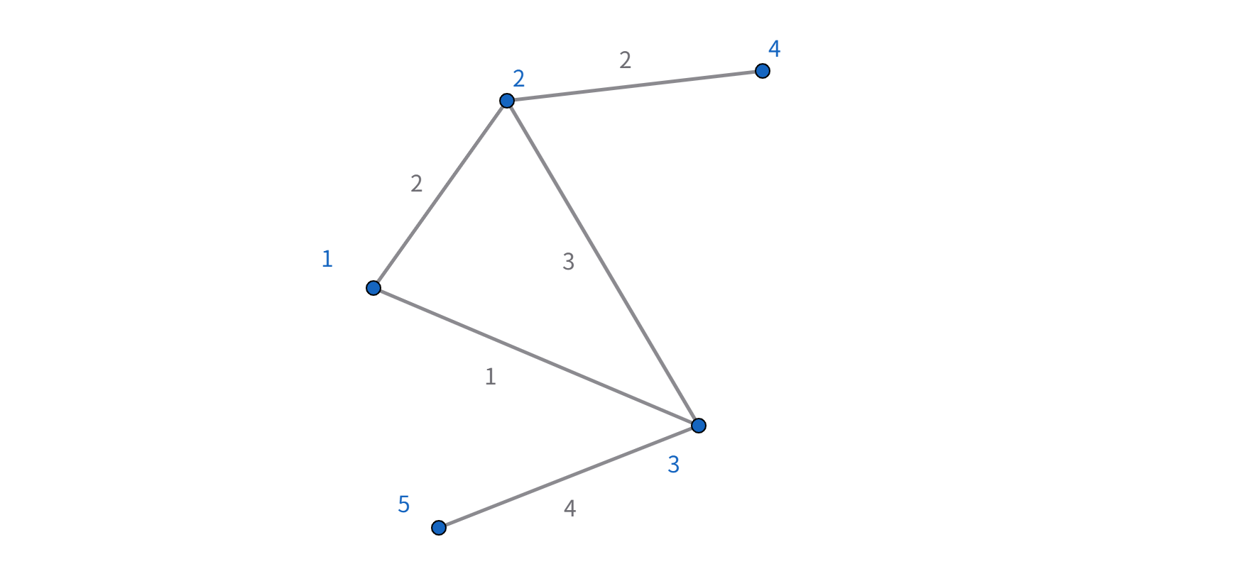
Edges are weighted as follows:
- (0,1): 2
- (0,2): 1
- (1,2): 3
- (1,3): 2
- (2,4): 4
We’ll represent the graph using an adjacency matrix \(W\), and compute the Laplacian matrix \(L = D - W\).
Step 1: Enumerate all configurations
Each node $i$ has a decision variable \(x_i \in \lbrace -1, 1\rbrace\). For \(n = 5\), there are \(2^5 = 32\) possible configurations.
For each configuration vector \(x = [x_0, x_1, …, x_4]\), we compute the cut value using the NLIP objective:
$$ f(x) = \frac{1}{2} \sum_{i,j} w_{ij}(1 - x_i x_j) $$
Or equivalently:
$$ f(x) = x^\top L x $$
Step 2: Find the best cut
We compute \(f(x)\) for each \(x \in \lbrace -1,1 \rbrace^5\) and record the one with the highest value. This is the exact solution to the NLIP.
Here’s a simplified version of the brute-force Max-Cut solver for small graphs:
for x_tuple in product([-1, 1], repeat=5):
    x = np.array(x_tuple)
    cut_value = x @ L @ x
    if cut_value > best_cut_value:
        best_cut_value = cut_value
        best_x = x.copy()
And the output will be:
Best cut value: 44
Best configuration: [-1  1 -1 -1  1]
What does this show
This approach works for small $n$—but even with just 5 nodes, we already have 32 configurations. For 10 nodes, that number jumps to 1024. For 20, over a million.
This illustrates the combinatorial explosion inherent in NLIP problems, especially when the variables are binary. While the formulation is clean and expressive, solving it exactly becomes infeasible very quickly.
In the next section, we’ll look at how semidefinite programming (SDP) provides a convex relaxation to approximate the solution in a much more scalable way.
3. SDP Relaxation of Max-Cut
The Max-Cut problem is inherently non-convex due to the \(\lbrace -1, +1\rbrace^n\) constraints on the variables. But there’s a well-known convex relaxation introduced by Goemans and Williamson (1995) that turns the NLIP into a semidefinite program (SDP).
The key idea is to replace the discrete variable vector \(x \in \lbrace -1, 1\rbrace^n\) with a rank-one matrix \(X = x x^\top\), where \(X \in \mathbb{R}^{n \times n}\) is symmetric and satisfies:
- \(X \succeq 0\) (i.e., \(X\) is positive semidefinite),
- \(\text{diag}(X) = 1\) (since \(x_i^2 = 1\) for all \(i\)),
- but we relax the rank constraint (drop \(\text{rank}(X) = 1\)).
The resulting SDP formulation is:
$$ \text{maximize} \quad \frac{1}{2} \sum_{i,j} w_{ij}(1 - X_{ij}) $$ $$ \text{s.t.} \quad X \succeq 0, $$ $$ \quad \quad \quad \text{diag}(X) = 1 $$
This is a convex optimization problem and can be solved efficiently using an SDP solver like MOSEK through Python with CVXPY. Here’s a basic implementation for a small graph:
# Define variable: symmetric PSD matrix X
X = cp.Variable((n, n), PSD=True)

# Objective: maximize (1/4) * sum w_ij * (1 - X_ij)
objective = cp.Maximize(0.25 * cp.sum(cp.multiply(W, 1 - X)))

# Constraints: diag(X) = 1
constraints = [cp.diag(X) == 1]

# Solve with MOSEK
prob = cp.Problem(objective, constraints)
prob.solve(solver=cp.MOSEK)

print("SDP objective value:", prob.value)
X_opt = X.value
And the output is:
SDP objective value: 10.999999924730195
This gives us a symmetric matrix \(X^\ast\) that satisfies the semidefinite and diagonal constraints. But it’s not yet a valid Max-Cut solution — we need to extract a cut from it. To get back to a valid \(\lbrace -1,1 \rbrace\) vector (i.e., a real cut), like in the textbook we proposed a randomized rounding method:
Step 1: Factor \(X^\ast\) into \(V V^\top\) (e.g., via Cholesky or SVD), where each row of \(V\) corresponds to a node.
Step 2: Generate a random hyperplane through the origin. Pick random vector \(r=(r_1,…,r_n)\), where draw each component \(r_j\) from \(\mathcal{N}(0,1)\).
Step 3: Assign each node \(i\) to side \(+1\) or \(-1\) based on which side of the hyperplane \(v_i\) falls on.
i.e., for each vertex \(i\):
- assign \(i\) to \(U\) if \(v_i \cdot r \geq 0\);
- assign \(i\) to \(W\) if \(v_i \cdot r < 0\).
This procedure gives a feasible cut (i.e., a valid \(\lbrace -1,1 \rbrace\) assignment), which can then be evaluated using the original Max-Cut objective.
In practice, the randomized rounding is repeated multiple times, and the best result is selected. And from the textbook we know the approximation ratio is around \(0.878\). If given the unique games conjecture there is no \(\alpha\) - approximation algorithm for Max Cut problem with \(\alpha \geq 0.878\) unless \(P = NP\).
4. If it is a good way of solving general NLIP?
The success of the SDP + randomized rounding approach for Max-Cut naturally raises the question: If it is a good way of solving general NLIP? And the first exploration into this question is:
For an NLIP to be a good candidate for the SDP relaxation and randomized rounding approach, it should primarily have a quadratic structure with binary variables.
More specifically, we notice that the Max Cut problem has the following ideal structure:
$$ \text{maximize/minimize} \quad x^T Q_0 x + c_0^T x $$ $$ \text{s.t.} \quad x^T Q_k x + c_k^T x \leq b_k \quad \text{for} \quad k=1,…,m $$ $$ \quad x_i \in \lbrace 0,1 \rbrace \quad \text{or} \quad x_i \in \lbrace -1,1 \rbrace \quad \text{for all i} $$
This class of problems are known as Quadratically Constrained Quadratic Programs(QCQPs), particularly when the variables are binary. And they are the most successful applications of this method. Max Cut is one of the most famous example and the one that pioneered this technique.
The magic of the SDP approach lies in its ability to “lift” the problem into a higher-dimensional space where it becomes convex. This works beautifully for quadratic terms.
5. Conclusion
In this post, we started from a classical nonlinear integer problem—Max-Cut—and explored how semidefinite programming (SDP) combined with randomized rounding offers a powerful way to approximate its solution. We walked through the modeling, the exact brute-force method, and then the elegant SDP relaxation that transforms the problem into a convex one.
While this technique works particularly well for problems with quadratic structures and binary variables, like Max-Cut and other QCQPs, it’s not a universal tool for all NLIPs. Still, when applicable, SDP relaxations provide not only computational efficiency but also meaningful approximation guarantees—something that’s rare in the world of combinatorial optimization.
Overall, Max-Cut serves as a perfect case study to understand a broader idea: sometimes the best way to approach a hard discrete problem is to relax it, solve a smarter version of it, and then round your way back to a solution.